Effect of RF on the Beam

R. BAARTMAN
TRIUMF
Vancouver, B.C. Canada

January 1993

Contents

1  Introduction: Why use rf?
2  What happens at an rf gap?
    2.1  Transverse focusing
    2.2  RF acceleration
    2.3  Required rf acceleration
3  The rest of the machine
4  Longitudinal Dynamics
    4.1  Adiabaticity
    4.2  Transition
    4.3  More Longitudinal Dynamics
    4.4  More on Longitudinal Emittance
5  Summary
A  Notes and Bibliography
    A.1  Introduction: Why use rf?
    A.2  What happens at an rf gap?
        A.2.1  Transverse focusing
        A.2.2  RF acceleration
        A.2.3  Required rf acceleration
    A.3  The rest of the machine
    A.4  Longitudinal Dynamics
        A.4.1  Adiabaticity
        A.4.2  Transition
        A.4.3  More Longitudinal Dynamics
        A.4.4  More on Longitudinal Emittance
    A.5  Summary

1  Introduction: Why use rf?

Let's start right at the very beginning: Why use rf? In circulating machines, particles return to the same location so energy gain can only occur if (ò)[E\vec]·d[l\vec] ¹ 0. [Symbols not properly typeset? Try XML version instead.] But we know that (ò)[E\vec]·d[l\vec]=0 for a static electric field [E\vec]. Hence, if we create a (static) potential drop across a gap, the energy gain is lost coming back to the same gap.
Therefore a time-varying field is needed in recirculating machines. In that way a localized electric field and energy gain can be achieved even though the electric potential is ground on either end of the gap. In linear machines which accelerate particles to energies larger than a few MeV, time-varying fields are needed as well. This is because it is not possible to maintain and control a potential drop of more than a few MV.
q1.png
We write down Maxwell's equation Ñ×[E\vec]=-[([B\vec])/(t)] (MKS units) in integral form:
ó
(ç)
õ

®
E
 
·d
®
l
 
= -

t
ó
õ
®
B
 
·
®
n
 
 dA.
(1)
So it turns out that to achieve an energy gain on a fixed orbit we need a time-varying magnetic field.
Naturally, [B\vec] and [E\vec] cannot grow to infinite levels so the time variation is oscillatory. (This also means that the beam will be bunched.) Moreover, the oscillation is generally sinusoidal because the most efficient way to generate strong electric fields is with a resonant cavity operating at one frequency.
But one may be wondering about the time-varying magnetic fields in synchrotron magnets: Do these contribute to the energy gain? Yes, but even in the fastest cycling synchrotrons it turns out to be a small effect. On the other hand, this effect is exploited in betatrons, which can be thought of as transformers with free electrons as the secondary winding.
Ex: Estimate the energy gain per turn due to this betatron effect in a small rapid-cycling synchrotron: frep=60 Hz, B in the dipoles varying from 0 to 2 Tesla, 200 m orbit length, half-filled with dipoles, each having a field occupying 20 cm. (Answer: a few kV.) Does it make any difference if C-magnet dipoles have their yokes inside or outside the beam orbit? The highest energy betatron is 300 MeV. Why are higher energies impractical?
In the remainder of this note, I deal with the effect of the rf gap on beam particles, the effect of the lattice on how beam particles move with respect to each other, and finally a description of the longitudinal dynamics resulting from the combination of these effects. The main emphasis will be on proton synchrotrons, but the discussion will be generalized wherever possible.

2  What happens at an rf gap?

q3.png
Two things happen to a particle crossing an RF gap: it gains energy (the intended effect), and it receives a transverse kick. We deal with the second one first.

2.1  Transverse focusing

Usually an rf gap is circular or at least elliptical in a plane perpendicular to the beam direction. With this kind of symmetry, it is clear that an on-axis particle receives no transverse kick. In the static-field case, an accelerated particle experiences a radial (focusing) electric field at the gap entrance, and a radial field of opposite sign (defocusing) at the exit. This adds up to a net focusing effect since the particle gains speed and so spends less time in the defocusing field than in the focusing field. It turns out that this effect is weak when rf acceleration is used because the fractional velocity gain is generally very small, and because a more important effect arises from the fact that the electric field itself is changing during the gap passage. Perhaps surprisingly, this latter effect does not depend upon gap length because a shorter gap of the same energy gain has proportionately stronger radial electric fields.
As stated, we assume the gap has mirror symmetry in the transverse coordinates x and y. We also assume small x and y (compared with the beam pipe radius) so that the fields are linear: Ex=[(Ex)/(x)]x and Ey=[(Ey)/(y)]y. The dynamics are simply: Fx=eEx=m[x\ddot]=mv2x" so that the change in x¢ during gap passage is 1
dx¢= ó
õ
x"dz= e

mv2
ó
õ
Exdz
(2)
and similarly for y. It is also a good approximation to assume that the gap is `thin' i.e. the particle does not move transversely during the gap passage. Then
dx¢= e

mv2
ó
õ
Ex

x
xdz » ex

mv2
ó
õ
Ex

x
dz.
(3)
In terms of the gap focal length fx=x/dx¢, we get:
1

fx
= e

mv2
ó
õ
Ex

x
dz and similarly, 1

fy
= e

mv2
ó
õ
Ey

y
dz.
(4)
If we add the two and use Ñ·[E\vec]=0, we find
1

fx
+ 1

fy
= - e

mv2
ó
õ
Ez

z
dz.
(5)
The integral is to be performed as a path integral on the (z,t)-plane since both z and t change as the particle moves.
dEz= Ez

z
dz+ Ez

t
dt.
(6)
So
1

fx
+ 1

fy
=- e

mv2
æ
è
ó
õ
dEz- ó
õ
Ez

t
dt ö
ø
.
(7)
The first integral vanishes because Ez is zero outside the gap. We introduce the harmonic variation of the electric field as Ez(t)=[^(Ez)]sinwt, differentiate w.r.t. t, and convert back into an integral over z by introducing the particle's phase f: wt=f+wz/v.
1

fx
+ 1

fy
= e

mv2
ó
õ
^
Ez
 
wcoswtdt = ew

mv3
ó
õ
^
Ez
 
cos(f+wz/v)dz.
(8)
The quantity wz/v varies by wg/v through the gap (g is the gap length). This is the gap transit angle: it is dealt with below and we show that it is a small number, so we ignore wz/v in the present context. The remaining integral, ò[^(Ez)]dz, is conventionally (for obvious reasons) called the voltage across the gap, V or Vrf. The final result is
1

fx
+ 1

fy
= ew

mv3
Vcosf.
(9)
In fact this is not relativistically correct, or, in other words, only applies in the reference frame of the particle. If we transform to the lab frame, we find that besides the 1/g factor due to replacing m by gm, there is a time dilation factor 1/g2. The final relativistically correct result is
1

fx
+ 1

fy
= ew

mb3g3c3
Vcosf.
(10)
The derivation may make one suspicious since the rf magnetic field has not been explicitly taken into account. As a matter of fact, it is included in the 1/g2 time dilation factor.
Ex: For a circular gap, find the rf magnetic field and show that the contribution it makes via [F\vec]=e[v\vec]×[B\vec] to dx¢ is -b2 times the electric contribution. This changes the total contribution by the factor 1-b2=1/g2.
For a circular gap as is generally the case in linacs and synchrotrons, fx=fy=f so we have
1

f
= 1

2
ew

mb3g3c3
Vcosf.
(11)
In a cyclotron, the gap is flat to allow the beam to gain in orbit radius, so there are no radial rf forces and 1/fx=0:
1

fy
= ew

mb3g3c3
Vcosf.
(12)
In any case, the focusing effect is largest at low energy, and at high rf frequency and voltage.
Ex: The following accelerators are all proton machines i.e. mc2=938/,MeV.
(1) In a typical proton synchrotron, w =2p×50 MHz, V=100 kV (per cavity), kinetic energy, T=600 MeV at injection so b =0.79 and g =1.64. This gives f=39 km: not an important effect.
(2) In the LAMPF drift tube linac at injection, rf frequency is 200 MHz, V is around 1 MV, and T=750 keV at injection. This gives f=3 cm: clearly an important effect.
(3) In the TRIUMF cyclotron, injection is at 300 keV, V=200 keV, and the rf frequency is 23 MHz. This gives f=15 cm, and since there is little magnetic focusing near injection (the machine centre), this is a large effect. As a matter of fact, the rf (de)focusing prohibits operating with f less than 90°.
Generally, the transverse rf focusing is important in cyclotrons and in proton linacs. In electron linacs, g is usually so high that the gap focusing is not important.
For a net focusing effect, we want 1/f to be negative. This requires f to be between 90° and 270°. Recall that this arises because the focusing is related to the time derivative of the electric field. Hence the central ingredient for net transverse rf focusing is a falling electric field2.

2.2  RF acceleration

As a particle drifts through the rf gap's electric field, it gains energy. Assume (for simplicity) that the gap has length g and the longitudinal electric field is uniform. Then
Ez= V

g
sinwt,
(13)
and the energy gain is eòEzdz, or
dE= eV

g
ó
õ
g/2

-g/2 
sinwtdz.
(14)
As before, the particle's motion is simply dz/dt=v, or, wt-wz/v=constant and we call this constant the phase f. Then
dE= eV

g
ó
õ
g/2

-g/2 
sin(wz/v+f)dz = eVsinf é
ë
sin(q/2)

q/2
ù
û
,
(15)
where q = wg/v is called the gap transit angle, and the factor in square brackets is called Tt, the transit time factor.
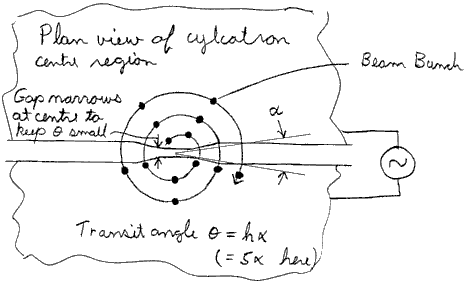
Ex: We go through the same three examples.
(1) In a typical proton synchrotron, w =2p×50 MHz, g=4 cm, and at T=600 MeV v=0.8c, giving q = 0.05 and Tt=0.99989: a small effect.
(2) In a drift tube linac we can think of setting the drift tube length approximately equal to the gap g. This automatically means q = p, and Tt=0.6. In this case it is clearly advantageous to make the gap as small as possible (up to the sparking limit).
(3) In cyclotrons, q is simply the angle subtended by the rf gap, multiplied by h, the harmonic number, i.e. the number of times the rf electric field oscillates during one revolution of the particle (more about this quantity later). In the case of TRIUMF, h=5. In order to keep Tt near 1, the gap is narrower at the centre of the machine than elsewhere. This is shown in the following sketch.
q7.png

2.3  Required rf acceleration

In electron linacs and cyclotrons the energy gain is not critical and so the particles are usually bunched near a phase of 90°.
In synchrotrons and in proton linacs the required energy gain per turn is given. In synchrotrons, a particle must gain the right energy to maintain proportionality between its total momentum and the magnetic field in the beam bending and focusing devices. In linacs, the energy gain is fixed by the drift tube and/or cavity geometry.
Since the energy gain is Vsinf, only one phase gains the prescribed energy. We call this the synchronous phase, fs. Just as it is not realistic to have all particles on the beam axis (zero transverse emittance), it is also not realistic to have all the particles at one phase (zero longitudinal emittance). For linacs, it is clear that the leading particles should receive a smaller energy gain than the lagging ones. Therefore, the electric field needs to be rising as the bunch of particles passes through the gap.
q8.png
Unfortunately, this is just the opposite of the condition for transverse rf focusing. Therefore it is not possible to construct a proton linac which depends only on the rf fields for both longitudinal and transverse focusing. It is amusing to blame Murphy for this state of affairs, but there is a simple physical explanation. Recall that in the reference frame of the synchronous particle, the transverse focal powers are [1/(fx)] = [e/(mv2)]ò[(Ex)/(x)]dz and similarly for 1/fy. In just the same way, one can define a longitudinal focal power [1/(fz)]=[(dz¢)/z] = [e/(mv2)]ò[(Ez)/(z)]dz, where z and z¢=Dp/p are measured with respect to the synchronous particle. But then it follows from Ñ·[E\vec]=0 that 1/fx+1/fy+1/fz=0 in the reference frame of the bunch, or, transformed to the lab frame,
1

fx
+ 1

fy
+ 1

g2fz
=0,
(16)
which means that fx, fy, and fz cannot all be simultaneously negative. So Murphy's law turns out to be a corollary of Gauss' Law.
Ex: Find 1/fz directly without using the above result, but by finding the difference between Dp/p for an arbitrary particle and for the synchronous particle.

3  The rest of the machine

What happens to the particles (longitudinally) as they are brought (back) to the (next) rf gap? In linacs, we already know the answer: particles with higher energy than required for synchronism will tend to move ahead of the synchronous particle and will come to the gap too soon. In recirculating machines, the story is a little more complicated.
First, we need to define a little more carefully what is meant by a particle's phase. It is the time with respect to the rf voltage that the particle passes through the rf gap.
We've already stated that the `right' energy gain is given; dE =Vsinfs, so the synchronous particle has phase fs. Moreover, it stays synchronous by also having the right energy Es (and hence the right velocity vs) so that the rf goes through an integer number of cycles as it comes back to the same gap.
The synchronous particle velocity is vs=dz/dt so that its longitudinal position along the equilibrium orbit is zs=vst+zs0. Say the rf gap is at z=0. Then the time of crossing the rf gap is -zs0/vs, or, in units of rf radians,
wrft=-zs0wrf/vs=fs.
(17)
Similarly, the ith particle has velocity vi, position zi=vit+zi0, and crosses the rf gap at time t=-zi0/vi, making its phase
fi=-zi0wrf/vi.
(18)
For the moment, we are concentrating on a one-cavity machine, so the drift distance for the synchronous particle to get back to the same gap is L, the length of the equilibrium orbit i.e. the machine circumference. The phase of the synchronous particle is then wrf t=(L-zs0)wrf/vs=Lwrf/vs+fs. To stay synchronous, this phase must be equal to an integer times 2p. We call this integer h, the harmonic number. Hence, the synchronism condition is Lwrf/vs=2ph. Since 2pvs/L is wrev, the revolution frequency of the synchronous particle, another way of writing the synchronous condition is wrf =hwrev.
Similarly, for the non-synchronous, ith particle, the phase change between successive crossings of the same gap is df = Liwrf/vi. The length of the ith particle's orbit, Li, is not the same as L because, as we shall see below, an off-momentum particle does not travel on the equilibrium orbit. We write vi=vs+Dv and Li=L+DL and assume the increments to be small quantities. Then we get df = 2ph(1-Dv/v)(1+DL/L), or, modulo 2p and ignoring second order terms, df = 2ph(DL/L-Dv/v). Since this is a small change and occurs during a time increment 2p/wrev =2ph/wrf, we get
1

wrf
df

dt
= DL

L
- Dv

v
.
(19)
A bit of relativistic kinematics shows that Dv/v =(1/g2)Dp/p. (This is the same 1/g2 factor that came up in the context of calculating rf focusing.) It turns out that DL/L is also proportional to Dp/p and the proportionality constant is called the momentum compaction factor ac. Therefore we can write
1

wrf
df

dt
= æ
è
ac- 1

g2
ö
ø
Dp

p
.
(20)
From whence comes this extra orbit length for the off-momentum particle? Let us imagine the simplest of all lattices; a single flat dipole. We know that the orbit radius r is given by Br = p/e, so the orbit length is L=2pr µ p. Hence, DL/L =Dp/p and ac =1. But this is for a flat dipole. In principle we can tailor the magnetic field so that it rises with momentum. If B(r) µ g then since L µ p/B, dL/L=dp/p-dg/g =(1-b2)dp/p=(1/g2)dp/p. Then df/dt=0, which means the machine is isochronous. This is the case in an isochronous cyclotron, and also momentarily in a synchrotron at transition.
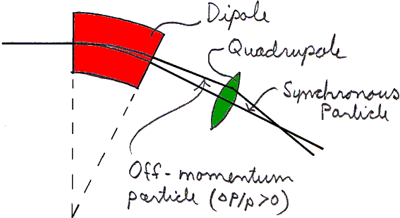
Ex: The isochronism condition is more simply v/r=constant. Use this to prove B=gB0, where B0 is a constant.
In synchrotrons (and synchro-cyclotrons), wrf is varied with time to stay in step with the accelerating beam. Therefore there is no isochronism constraint. Generally, dipoles (usually flat, but not necessarily) are interspersed with quadrupoles so that the off-momentum particle follows some convoluted orbit.
q10.png
The lattice designer can in principal come up with almost any momentum compaction, even a negative one. In the simplest, most regular lattices, ac » 1/nx2 where nx is the number of horizontal oscillations a particle makes about the equilibrium orbit (the horizontal `tune'). For cyclotrons, this means nx » g, making it impossible to avoid betatron resonances in high energy cyclotrons. On the other hand, in fixed orbit machines i.e. synchrotrons, ac does not vary with energy. This is unfortunate because it means that the factor
h = df

d(wrft)
/ Dp

p
=ac- 1

g2
(21)
changes as the particle accelerates, and may even go through zero. This factor is called the `phase slip' factor and as we shall see, it determines the longitudinal focusing.
To summarize, in cyclotrons the longitudinal focusing does not vary with energy, but the horizontal focusing does. In synchrotrons, the horizontal focusing does not vary with energy but the longitudinal focusing does. In linacs we can also define a phase slip factor. (Though we've used L as the orbit length, it is clear that the definition can be generalized to mean the distance between rf gaps.) Since there are no bending magnets, ac =0, so in electron linacs, where g is very large, h is practically zero.
Accelerator momentum phase slip
type comp. ach
Proton linac 0 -1/g2
Electron linac0 0
Cyclotron 1/g20
Synchrotron fixed by latticeac-1/g2

4  Longitudinal Dynamics

Now we are in a position to describe the longitudinal dynamics. The synchronous energy gain is dEs=Vsinfs, while that for an arbitrary particle with phase f is dE =Vsinf. Hence, the per-turn change in energy deviation DE =E-Es is
d(DE)=V(sinf-sinfs).
(22)
From relativistic kinematics, DE =b2gE0(Dp/p), where E0 is mc2, the rest mass. So we write
d æ
è
Dp

p
ö
ø
= V

b2gE0
(sinf-sinfs).
(23)
This change is small, and since it occurs during a time increment of 2ph/wrf, we write it as
d

d(wrft)
æ
è
Dp

p
ö
ø
= V

b2gE0
sinf-sinfs

2ph
.
(24)
Recall that
df

d(wrft)
= æ
è
ac- 1

g2
ö
ø
Dp

p
=h Dp

p
.
(25)
We combine these into
d2f

dt2
= wrf2hV

2pb2gE0h
(sinf-sinfs).
(26)
This is a nonlinear oscillator, but we concentrate on cases where f departs only slightly from fs; i.e. f = fs+Df where Df is small. Expanding sinf, we find sinf » sinfs+Dfcosfs, giving the linearized equation
d2Df

dt2
+ é
ë
wrf2(-h)Vcosfs

2pb2gE0h
ù
û
Df=0.
(27)
This is a simple harmonic oscillator. Oscillations are stable if the quantity in square brackets is positive: the square root of this quantity is the (angular) frequency of the oscillations, wf.
For h < 0 i.e. g < ac-1/2 º gt, we must have cosfs > 0, or, -p/2 < fs < p/2, which is the same as saying that the voltage across the gap must be rising as the particles pass.
q12.png
This is a conclusion we already made for linacs. The regime h < 0 is called `below transition'. Physically, in this regime the particle energy is sufficiently low that higher velocity of the higher energy particle dominates over the longer path in determining the revolution period.
Conversely, above transition the stable phase must be between p/2 and 3p/2 to make cosfs < 0. For acceleration, we also require sinfs > 0 so fs must be between p/2 and p. Physically, in this regime leading particles get a relatively larger energy gain. This makes them take a longer path around the machine so that by the time they come back to the rf gap they have fallen back a little towards the synchronous phase.
Ex: Fermilab Booster; h=84, gt =5.4 i.e. ac =0.034. At injection, T=200 MeV, V=275 keV, fs =0 (just before acceleration starts), and the rf frequency is 30 MHz. Find the phase oscillation frequency ff=wf/(2p). At extraction, just as acceleration ends, T=8 GeV, the rf frequency is 53 MHz and V=380 kV. What is fs? Find frf and ff. Also find the `synchrotron tune' ff/frf in both cases.

4.1  Adiabaticity

Some of you will (rightly) complain that the equation of motion is not simple harmonic since V, fs, and g all vary with time so wf varies with time. It turns out that the analysis is still correct if the variation is slow enough, or, `adiabatic'. How slow is `slow'?
Clearly, the time scale is given by the reciprocal of wf =2pff. If
d

dt
æ
è
1

wf
ö
ø
<< 1,
(28)
then the motion is adiabatic. This is a fuzzy concept: how much less than 1 depends upon how much spoilage of beam quality is tolerated. We will get into a definition of beam quality later, but for the moment will put up with the fuzziness.
Ex: In the Fermilab Booster, say we want to drop V by 100 kV at extraction. How quickly can this be done? In the SSC LEB, matching the beam to the MEB requires dropping the rf voltage a factor of 10 in the last millisecond. But at extraction ff is very low, around 500 Hz, because h is very small. Will the motion be adiabatic during this change?

4.2  Transition

In machines with regular lattices, gt » nx. Since the tune is on the order of 10, this means that if such a machine accelerates protons through an energy on the order of 10 GeV, it will accelerate through transition. (Electron machines with their high g always are above transition.) This means not only that the rf phase needs suddenly to be switched from fs to p-fs, but also that wf goes momentarily to zero. It is reasonable to expect an adiabaticity problem near transition, but on the other hand, with wf small the longitudinal motion is so slow that perhaps there is no problem. This is clearly a special case and needs a closer look.
Recall the linearized equations of motion
d

d(wrft)
(Df)=h Dp

p
,
(29)
and
d

d(wrft)
æ
è
Dp

p
ö
ø
= Vcosfs

b2gE0
Df

2ph
.
(30)
Multiply the first by 2Df and the second by 2Dp/p:
d

d(wrft)
(Df)2=h æ
è
Dp

p
Df ö
ø
,
(31)
and
d

d(wrft)
æ
è
Dp

p
ö
ø
2

 
= Vcosfs

2pb2gE0h
æ
è
Dp

p
Df ö
ø
.
(32)
Combined, these give
d

d(wrft)
é
ê
ë
(Dp/p)2

Vcosfs

2phb2gE0
+ (Df)2

-h
ù
ú
û
=0,
(33)
so the quantity in square brackets is constant. This means that the particles travel on ellipses in Df-Dp/p-space (otherwise known as longitudinal phase space).
q14.png
They travel with angular frequency wf and the ellipse has aspect ratio
^
Dp/p

^
Df
=   æ
Ö

Vcosfs

2ph(-h)b2gE0
 
= wf

hwrf
.
(34)
It turns out that the area of this ellipse, namely, p[^(Df)][^(Dp/p)] is an adiabatic invariant and its adiabaticity depends on the aspect ratio varying sufficiently slowly. We will not prove this statement here, but one can see for example that if a particle is at the extreme phase extent of its orbit (Dp/p =0) and the aspect ratio is instantaneously changed (say by changing the rf voltage), then the particle will follow a new ellipse of different area. It is this area (actually, that corresponding to the trajectory of the outermost particle in the bunch), which quantifies the previously-introduced notion of beam quality. It is called the longitudinal emittance.
Ex: Generally, the longitudinal emittance is given in energy-time units as ef =p[^(DE)][^(Dt)]. The conversion from one system of units to the other is left as an exercise to the reader. Ans:
ef= b2gE0

wrf
æ
ç
è
p
^
Dp

p
 
^
Df
 
ö
÷
ø
(35)
So from eqn. 34 it is not wf, but wf/h whose slowness of variation determines the adiabaticity. This means that transition crossing is not necessarily non-adiabatic. For adiabaticity, we would like the quantity [(Vcosfs)/(2ph(-h)b2gE0)] to be constant near transition, but at the same time, the magnets continue ramping up and so the energy gain dE =Vsinfs is a given constant as well. Together, these determine both V and fs as a function of time through transition:
cotfs=-Kh
(36)
where K=2phb2gE0/dE, and
V=dE
Ö
 

1+K2h2
 
.
(37)
What is happening during this type of crossing? Particles rotate in phase space on a constant ellipse, but rotation slows to a stop and reverses direction. This technique is called `duck-under' transition because the voltage waveform with respect to the bunch of particles looks as follows.
q16a.png
Does the technique work? In general, no. The reason is that there is still a time range near transition where wf is so small that the longitudinal motion becomes dominated by non-linearity, space charge, and other undesirable effects.
One of these effects is the non-linearity of the rf waveform. In connection with instabilities, we shall see that the non-linearity is usually beneficial. However, near transition, where fs =p/2, leading and lagging particles gain too little energy compared with the particles near the centre of the bunch. This leads to the type of distortion shown below.
q16b.png
The change in the path length with energy contains nonlinear terms, and near transition the linear term in the phase slip has vanished. Thus, there will be a distortion where particles with large |Dp/p| slip in phase with respect to the particle with small momentum deviation. This leads to the type of distortion shown below.
q17a.png
A third type of distortion comes from space charge. Ordinarily, it primarily results in a slight change in the phase space ellipses' aspect ratios. At transition, however, the leading particles will gain energy due to the repulsion by the rest of the bunch, while lagging particles lose energy. Moreover, the energy change is not linear because particles in the sparse regions at the extreme head and tail of the bunch see no space charge field. Schematically, the distortion looks as shown below.
q17b.png
Cyclotrons operate continuously at transition. How do they deal with these problems? They use an additional rf harmonic (usually third) to flattop the energy gain.
q18.png
This solves the first two of the afore-mentioned distortions, and, by phasing the additional harmonic to tilt the flattop, can at least correct the linear part of the space charge effect. This is a new idea for synchrotrons (suggested by Jim Griffin). Shortly before transition, a third harmonic cavity is ramped up to approximately 1/8 the voltage of the fundamental, and shortly after transition it is ramped back down and switched off. The time interval over which this is to occur is simply that during which the nonlinear effects are not small with respect to the linear forces.
Of course we can avoid the problem entirely by manipulating the lattice design to move gt outside the range of beam g during acceleration. This is the approach taken in the KAON Factory rings and in the SSC LEB. In the 30 GeV KAON Factory ring design, gt has been moved beyond infinity to an imaginary value. This means that ac < 0 so that higher energy particles take a shorter path around the machine.

4.3  More Longitudinal Dynamics

Let us investigate the non-linear longitudinal motion. We multiply both sides of
d

d(wrft)
æ
è
Dp

p
ö
ø
= V

b2gE0
sinf-sinfs

2ph
(38)
by df and integrate:
R.H.S.
=
V

2phb2gE0
[constant-(cosf+fsinfs)],
(39)
L.H.S.
=
ó
õ
df

d(wrft)
d æ
è
Dp

p
ö
ø
= h ó
õ
æ
è
Dp

p
ö
ø
d æ
è
Dp

p
ö
ø
= h

2
æ
è
Dp

p
ö
ø
2

 
.
(40)
Therefore,
1

2
æ
è
Dp

p
ö
ø
2

 
+ V

2ph(-h)b2gE0
[(cosfs+fssinfs)-(cosf+fsinfs)] = K2

2
,
(41)
where K is a constant. For small Df =f-fs, this reduces to elliptical orbits in phase space as we found previously (33). So the orbits are ellipses at small amplitudes, becoming distorted at larger amplitudes. If a particle's amplitude is such that it reaches the phase p-fs at Dp/p =0, then it will stall at that point, because, as we have seen, this is a fixed point, but an unstable one. The trajectory which passes through this point is called the `separatrix' because it separates the stable area in phase space, where the motion is bounded, from the unstable area, where the motion is unbounded. The stable area in phase space is referred to as the `bucket'.
q19.png
The distortion causes the synchrotron frequency wf to fall with amplitude, becoming zero on the separatrix. There is no analytic formula for the frequency variation (except when fs =0), but one can perform an expansion. The first two terms are (trust me)
wf(
^
Df
 
) = wf(0) é
ê
ë
1- æ
è
1+ 5

3
tan2fs ö
ø
^
Df
 
2
 

16
ù
ú
û
.
(42)
This constitutes a frequency spread for the bunch of particles and is a good thing because it can damp out and stabilize otherwise-unstable collective effects. Physically, the particles cannot sustain a coherent error signal because they will go out of step in a time interval of approximately 1/Dwf. But this also gives a time scale for correcting matching errors. We call a bunch `matched' if it has the same shape as the trajectories in phase space. A dipole mismatch is where the bunch is not centred on the synchronous phase. A quadrupole mismatch occurs if the beam aspect ratio is not the same as that of the orbit trajectories. Similarly, a sextupole mismatch is where the bunch has a somewhat triangular shape, and so on for octupole, etc. These are shown in the figure below, along with the effect of frequency spread, if these errors are not corrected quickly enough.
q20.png
It can be seen that in all cases the error, if uncorrected, results in an increase in beam emittance. A dipole mismatch can be corrected by controlling the rf phase. However, it must be borne in mind that if h > 1, there can be many circulating bunches, and each bunch may have a different phase error. Similarly, a quadrupole mismatch can be corrected by controlling the rf voltage in a loop with a sensor which detects length variations in the bunches. Higher order mismatches require more sophisticated schemes, and are generally not corrected.
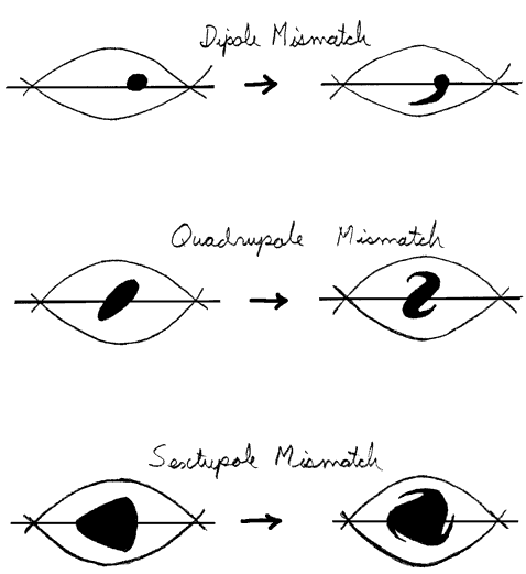
Ex: At injection, the TRIUMF Booster (proposed in 1989 but never built) has fs =0, [^(Df)]=100°, and wf =2p×50 kHz. Calculate the time interval over which mismatch errors must be damped. Ans: Must be short compared with 17 ms, i.e. a few turns (each turn is 1 ms).

4.4  More on Longitudinal Emittance

We already know that Vsinfs is fixed by the required energy gain per turn. If B is the field in a bending dipole, Br = p/e, where r is the bending radius. Therefore, dp/dt=erdB/dt. Since in one turn, Dp =DE/(bc)=Vsinfs/(bc) while Dt =L/(bc), we get
Vsinfs=erL dB

dt
.
(43)
We see that V must be larger than erLdB/dt, but by how much? We know that the voltage must be rising (falling) as the synchronous particle crosses the rf gap, when below (above) transition. Therefore, fs =p/2 is not allowed. Recall also that the beam (longitudinal) emittance is an adiabatic invariant. This means that the beam bunch occupies an incompressible area in phase space. For fixed Vsinfs, we can vary the rf voltage and receive phase-space buckets of the following shape.
q21.png
The point is that the larger the voltage, the larger the bucket area. One can calculate the area of the bucket and compare with the known required area corresponding to the beam emittance. However, this is not really the best approach because there is always a significant area near f = p-fs which is not useful: particles travelling through it come exceedingly close to the separatrix and slight variations (noise) in V can cause particles to fall out of the bucket. Besides, bucket area is not an analytically calculable parameter; one must look it up in tables or run a computer calculation involving numerical integration. What's really important is how closely the outside particle approaches the separatrix. This is easily calculated analytically.
From the equation of motion (38), we see that for any given orbit, maximum Dp/p occurs at f = fs. Therefore, maximum Dp/p is equal to K, with K given by eqn. 41. We know the separatrix passes through (f = p-fs,Dp/p =0) so, again from eqn. 41, we find that the maximum Dp/p in the bucket is
Dp

p
ê
ê


bucket 
= 2   æ
Ö

Vcosfs

2ph(-h)b2gE0
 

Ö
 

1-(p/2-fs)tanfs
 
.
(44)
In the case of the beam, we have in the linear approximation,
Dp

p
ê
ê


beam 
=
  æ
Ö

æ
è
^
[(Dp)/p]
 
^
Df
 
ö
ø
æ
è
Dp/p

Df
ö
ø
 
=
  æ
Ö

ef

p
wrf

b2gE0
 
æ
è
Vcosfs

2ph(-h)b2gE0
ö
ø
1/4

 
.
(45)
We use the symbol Pf to denote what we call the `filling factor':
Pf= Dp/p|beam

Dp/p|bucket
=
  æ
Ö

ef

4p
wrf

b2gE0
 

æ
è
Vcosfs

2ph(-h)b2gE0
ö
ø
1/4


Ö
 

1-(p/2-fs)tanfs
 
.
(46)
Ex: Calculate the voltage V needed in the SSC Low Energy Ring (never built) at injection (600 MeV, fs =0) to accommodate ef =0.018 eVs with a filling factor of Pf=75 %. Other parameters are frf =50 MHz, h=114, and gt is very high (ac << 1/g2). Ans: 155 kV.
Notice that V µ 1/Pf4, so increasing the safety margin costs a lot in rf. Eg., decreasing Pf by 20% requires a twice larger rf voltage.
Given dE =Vsinfs, we can cast the last eqn. into the following slightly simpler form, useful for moving buckets (i.e. fs ¹ 0):
1-(p/2-fs)tanfs


Ö

-htanfs
= effrf

2Pf2
  æ
Ö

2ph

b2gE0dE
 
(47)
Note that this eqn. is correct on either side of transition, since -htanfs is always positive. The function on the L.H.S. (without -h) is plotted below.
q23.png
Ex: At mid-cycle in the SSC LEB, T=(g-1)E0=5.73 GeV, dE =0.611 MeV (comes from a total energy gain of 10.5 GeV in a sinusoidal acceleration ramp of 50 ms). For ef =0.02 eVs and Pf < 0.5, find the upper limit on fs and the lower limit on V. Ans: 52° and 770 kV.

5  Summary

We have learned how to calculate both longitudinal and transverse effects of rf gaps on the beam. We have studied longitudinal phase space dynamics and know how to calculate bucket parameters, required rf voltage and synchronous phase, even in the region near transition energy in a proton synchrotron.
One fact that has been ignored up to this point is that in general the required rf voltage and power is too much for a single cavity. In general, many rf cavities are required, and this opens up the possibility that they do not all have the same phase relative to the beam. This is an advantage when an anomalously low voltage is required (eg. to match the beam to a subsequent synchrotron), because cavities can be phased in opposition to avoid going to uncontrollably low rf voltages. The results obtained so far are correct even in this case, provided the individual gap voltages and phases are added vectorially, and provided that the quantity wf/wrev (called the `synchrotron tune') is much smaller than 1. This latter condition is true in general because other dynamical problems occur if it is violated.

A  Notes and Bibliography

As a general reference, one can use any introductory text or course on longitudinal beam dynamics.
For a more general, more mathematical treatment, consult the following.
Specific references for specific sections follow; the numbering scheme in this matches that of the main article.

A.1  Introduction: Why use rf?

A.2  What happens at an rf gap?

A.2.1  Transverse focusing

A.2.2  RF acceleration

A.2.3  Required rf acceleration

A.3  The rest of the machine

A.4  Longitudinal Dynamics

A.4.1  Adiabaticity

A.4.2  Transition

A.4.3  More Longitudinal Dynamics

I couldn't find a derivation of the synchrotron frequency as a function of amplitude, so here is my own.
We can start with Eqn. 41 and remember that Dp/p µ df/dt. Then it is clear that
æ
è
df

dt
ö
ø
2

 
µ  C+cosf+fsinfs.
(48)
The extremes f1 and f2 of the closed phase space trajectory occur when df/dt=0 so the constant C is given by
C+cosf1+f1sinfs=C+cosf2+f2sinfs=0.
(49)
The synchrotron period Tf is therefore given by
Tf µ ó
õ
f2

f1 
df


Ö

C+cosf+fsinfs
.
(50)
(We can worry about the proportionality constant later because we already know the synchrotron frequency for vanishing amplitude.) Now we expand f about fs, writing f = fs+d, f1=fs+d1, and f2=fs+d2. The expression under the square root sign becomes
C+cosfscosd+(fs+d-sind)sinfs » cosfs

2
é
ë
K2- æ
è
d2-tanfs  d3

3
- d4

12
ö
ø
ù
û
.
(51)
The new constant K2 retains the feature that this expression vanishes at the endpoints d = d1 and d = d2. The synchrotron period Tf can now be written
Tf µ ó
õ
d2

d1 
dd


Ö

K2-(d2-tanfs d3/3-d4/12)
.
(52)
Now for d2-tanfs d3/3-d4/12 we substitute K2sin2q. Then at d = d1, q = -p/2 and at d = d2, q = p/2. This converts the denominator into Kcosq, but we must now find an expression for dd/dq in terms of q. We write
d2=K2sin2q+tanfs  d3

3
+ d4

12
.
(53)
For d4 the lowest order approximation
d4=K4sin4q
(54)
is sufficient, but for d3, we need an expansion to two terms:
d2=K2sin2q+tanfs  d3

3
» K2sin2q æ
è
1+ tanfs

3
Ksinq ö
ø
,
(55)
so
d3=K3sin3q æ
è
1+ tanfs

2
Ksinq ö
ø
.
(56)
Now we substitute (54) and (56) into (53):
d2=K2sin2q æ
è
1+ tanfs

3
Ksinq+ 1+2tan2fs

12
K2sin2q ö
ø
.
(57)
To take the square root, we use the expansion Ö{1+x} » 1+x/2-x2/8 and find
d
=
Ksinq æ
è
1+ tanfs

6
Ksinq+ 1+2tan2fs

24
K2sin2q- tan2fs

72
K2sin2q ö
ø
=
Ksinq+ tanfs

6
K2sin2q+ 1

24
æ
è
1+ 5

3
tan2fs ö
ø
K3sin3q.
(58)
The integrand is therefore
dd

Kcosq
= æ
è
1+ tanfs

3
Ksinq+ 1+(5/3)tan2fs

8
K2sin2q ö
ø
dq,
(59)
and integrating from -p/2 to p/2, we get
Tf µ ó
õ
p/2

-p/2 
dd

Kcosq
= p é
ë
1+ æ
è
1+ 5

3
tan2fs ö
ø
K2

16
ù
û
.
(60)
It is clear from (58) that
d1
» -K
+ tanfs

6
K2,
(61)
d2
» K
+ tanfs

6
K2.
(62)
Hence,
K= d2-d1

2
= f2-f1

2
º
^
Df
 
.
(63)
(As an aside, we see that we have hereby also found the first order asymmetry of the motion of f about fs for fs ¹ 0: d1 ¹ -d2, but d1 » -d2+tanfs d22/3.) The change in synchrotron period and frequency with amplitude is given by
DTf

Tf0
= - Dwf

wf0
= æ
è
1+ 5

3
tan2fs ö
ø
æ
ç
è
^
Df

4
ö
÷
ø
2

 
.
(64)

A.4.4  More on Longitudinal Emittance

I don't know of any other derivation of eqn. 47 or a comparable formula.

A.5  Summary


Footnotes:

1Notation: We use d to denote particle parameter increments which occur at the rf gap. The large D is used to denote deviations of particle parameters from those of a reference particle.
2We are using a convention that a positive electric field accelerates the particle, whatever the sign of the particle's charge.


File translated from TEX by TTH, version 3.67.
On 22 Jan 2007, 16:52.